Building And Training Spiking Neural Networks From Scratch
by R Gaurav
In this tutorial, we will learn how to build a Spiking Neural Network (SNN) from scratch and directly train it via Surrogate Gradient Descent (SurrGD) method. This tutorial although fast paced, is meant for absolute beginners in SNNs, and requires a basic-to-intermediate understanding of PyTorch.
Introduction
Spiking Neural Networks (SNNs) are architecturally similar to the conventional ANNs/DNNs, however, built with spiking neurons instead of the conventional rate neurons (i.e., \(\texttt{ReLU}\), \(\texttt{Sigmoid}\), etc). This way, the SNNs are more biologically plausible than ANNs/DNNs.
Why SNNs? Because, apart from several other advantages, they are energy-efficient compared to the ANNs/DNNs, -- albeit on neuromorphic hardware; thus, a promising step towards Green-AI.
More reasons to adopt SNNs can be found here. There are two common approaches to build SNNs:
-
ANN-to-SNN: In this method, we first train the desired ANN/DNN via regular Back-propagation based methods, followed by its conversion to an isomorphic SNN. Unfortunately, this method usually results in SNNs which have higher inference latency. My Nengo-DL tutorials: (1) and (2) cover this ANN-to-SNN approach; other libraries offering ANN-2-SNN conversion exist too, e.g., SNN Toolbox and Lava (this one offers an improvement over the conventional ANN-to-SNN conversion). -
Direct Training: In this method, we directly train our desired SNNs using approaches inspired from Computational Neuroscience, Back-propagation, etc. Examples include Spike Timing Dependent Plasticity (STDP) based methods, Back-propagation Through Time (BPTT) based methods, etc. One such highly effective and popular method is BPTT-based Surrogate Gradient Descent (SurrGD), where the SNNs are trained using a surrogate-derivative function. We focus on the SurrGD method here and discuss it in more detail later.
Spiking Neuron
We first start by implementing a simple Spiking Neuron model (to be used in our SNN), followed by the actual implementation and training of a Dense-SNN (i.e., composed of Dense spiking layers only). A spiking neuron is a stateful system, such that it maintains an internal Voltage state (\(V\)) and outputs a discrete (usually binary) Spike (\(S\)) of magnitude \(1\) whenever its \(V\) reaches or crosses a set Threshold voltage (\(V_{thr}\)); once the neuron spikes, its \(V\) is reset to \(0\).
From a number of spiking neuron models, most popular ones suited for SNNs are Integrate & Fire (IF), and Leaky Integrate & Fire (LIF) neuron models. I have already implemented a detailed LIF neuron model in a previous tutorial; here we focus on the simpler IF neuron model to build our SNN.
Following is the continuous-time equation of the IF neuron model:
where \(C\) is the neuron’s Capacitance and \(I(t)\) is the input Current. Following is its discrete-time implementation (for computers), which I am using to build my Dense-SNN here:
where \(I[t]\), \(V[t]\), and \(S[t]\) are the dicrete notations of Current, Voltage, and Spike respectively; \(\Theta\) is the Heaviside step-function. Note that all the incoming spikes \(S_j[t]\) are weighted by the associated weights \(W_j\) and added to the decaying Current (\(\alpha < 1\) is the Decay constant).
Bonus: To adapt the above neuron model to a simple version of
LIF, simply decay the Voltage by another Decay constant, say \(\beta < 1\), i.e., \(V[t] = \beta V[t-1] + I[t]\).
Note: Some neuron implementations also account for the refractory period in their models. During the refractory period, the neuron’s \(V[t]\) remains at \(0\) for the chosen number of time-steps, and it is incapable of producing a spike!.
Implementation
Following is the code for implementing a single IF neuron model, whose threshold voltage (\(V_{thr}\)) is set to \(1\). It accummulates/integrates the input into its \(V[t]\) state, and generates a spike of magnitude \(1\) whenever \(V[t]\) reaches or crosses the \(V_{thr}\) – simultaneously, \(V[t]\) is reset to \(0\). Note that in the implementation below, I am also rectifying the state \(V[t]\) to \(0\), in case it goes negative.
class IF_neuron(object):
  def __init__(self, v_thr=1.0):
    """
    Args:
      v_thr <int>: Threshold voltage of the IF neuron, default 1.0 .
    """
    self._v_thr = v_thr
    self._v = 0

  def encode_input_and_spike(self, inp):
    """
    Integrates the input and produces a spike if the IF neuron's voltage reaches
    or crosses threshold.

    Args:
      inp <float>: Scalar input to the IF neuron.
    """
    self._v = self._v + inp
    if self._v >= self._v_thr:
      self._v = 0 # Reset the voltage and produce a spike.
      return 1.0 # Spike.
    elif self._v < 0: # Rectify the voltage if it is negative.
      self._v = 0

    return 0 # No spike.
Executing the IF neuron
# Import necessary libraries.
import numpy as np
import matplotlib.pyplot as plt
from nengo_extras.plot_spikes import plot_spikes
# Create one spiking neuron and encode a random input signal.
if_neuron = IF_neuron(v_thr=1) # Instantiate a neuron.
T = 100 # Set the duration of input signal in time-steps.
inp_signal = 2*(0.5 - np.random.rand(T)) # Generate signal.

spikes = []
for t in range(T): # Execute the IF neuron for the entire duration of the input.
  spikes.append(if_neuron.encode_input_and_spike(inp_signal[t]))
spikes = np.array(spikes).reshape(-1, 1)
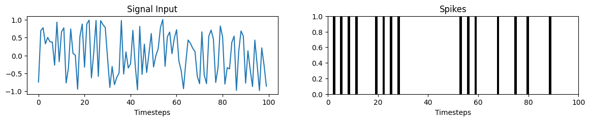
Plotting the input and generated spikes
plt.figure(figsize=(14, 2))
plt.subplot(1, 2, 1)
plt.plot(inp_signal)
plt.title("Signal Input")
plt.xlabel("Timesteps");
plt.subplot(1, 2, 2)
plt.title("Spikes")
plot_spikes(np.arange(0, T), spikes)
plt.xlabel("Timesteps");
plt.xlim([0, 100]);
Dense-SNN layers
Now that we have implemented a single IF neuron – the fundamental unit of an SNN, we next focus on building and training a Dense-SNN from scratch. The architecture here consists of an input Encoder layer, followed by two Hidden layers and a final Output layer (all the layers are spiking). We will use the MNIST dataset, which will be flattened for the input to our Dense-SNN. The Encoder layer rate encodes the normalized pixel values to binary spikes, upon which, the Dense connections in the Hidden layers learn the feature maps. The Dense connection in the Output layer then learns the classication over the feature map via the CrossEntropyLoss function.
Implementation
For convenience and uniformity of spiking layers in our SNN, I am first implementing the BaseSpkNeuron class, which can be inherited by the spiking Encoder, Hidden, and Output layers. The Output layer consists of spiking neurons equal to the number of classes. The mean of the output spike trains (over simulation time-steps) is passed to the loss function to compute classification error. I begin by importing the necessary libraries and defining the network constants:
import torch
from abc import abstractmethod
import numpy as np
import torchvision

V_THR = 1.0
DEVICE = "cpu" # Change it to "cuda:0" if you have an NVIDIA-GPU.
BATCH_SIZE = 500 # Change it to suit your memory availability.
TAU_CUR = 1e-3 # Time constant of current decay.
BaseSpkNeuron class
This class implements the basic template of IF spiking neurons arranged in a vector/matrix form. It will be inherited by other classes, which implement the Encoding and Spiking-Hidden layers.
class BaseSpkNeuron(object):
  def __init__(self, n_neurons):
    """
    Args:
      n_neurons: Number of spiking neurons.
      v_thr <int>: Threshold voltage.
    """
    self._v = torch.zeros(BATCH_SIZE, n_neurons, device=DEVICE)
    self._v_thr = torch.as_tensor(V_THR)

  def update_voltage(self, c):
    """
    Args:
      c <float>: Current input to update the voltage.
    """
    self._v = self._v + c
    mask = self._v < 0 # Mask to rectify the voltage if negative.
    self._v[mask] = 0

  def re_initialize_voltage(self):
    """
    Resets all the neurons' voltage to zero.
    """
    self._v = torch.zeros_like(self._v)

  def reset_voltage(self, spikes):
    """
    Reset the voltage of the neurons which spiked to zero.
    """
    mask = spikes.detach() > 0
    self._v[mask] = 0

  @abstractmethod
  def spike_and_reset_voltage(self):
    """
    Abstract method to be mandatorily implemented for the neuron to spike and
    reset the voltage.
    """
    raise NotImplementedError
In the above class definition, note that all the child classes must implement the spiking function in the spike_and_reset_voltage() as the Heaviside step-function, i.e., \(\Theta (x) = 1\) if \(x\geq0\) else \(0\). Since this step-function \(\Theta\) is discontinuous and non-differentiable at \(x=0\), (i.e., the derivative of \(\Theta(x)\) is the ill-defined Dirac’s \(\delta\) function), Back-propagation based methods to train the SNNs are not natively applicable. Note that the derivative \(\Theta^\prime(x)\) (\(=\frac{\partial \Theta(x)}{\partial x}\)) is \(0\) everywhere except at \(x=0\) where it is undefined. Thus, when applying Back-propagation natively, the error-gradients either vanish or explode, rendering the training of the weights infeasible. To alleviate this gradient vanishing/exploding problem, one needs to approximate the \(\delta\) function (i.e., \(\Theta^\prime(x)\)) via a surrogate-derivative function, explained below.
Surrogate Spike-Derivative
The concept of using a surrogate spike-derivative in place of the ill-defined \(\frac{\partial \Theta(x)}{\partial x}\) has been explored by a number of researchers to directly train the SNNs. Here I use the the partial derivative of the fast sigmoid function \(f(x) = \frac{x}{(1 + |x|)}\), i.e., \(f^\prime(x) = \frac{1}{(1+|x|)^2}\) as an approximation for \(\Theta^\prime(x)\) (as used by F. Zenke – basis of this tutorial). The figure below shows the plot of \(f(x)\) in red, and of \(f^\prime(x)\) in purple.
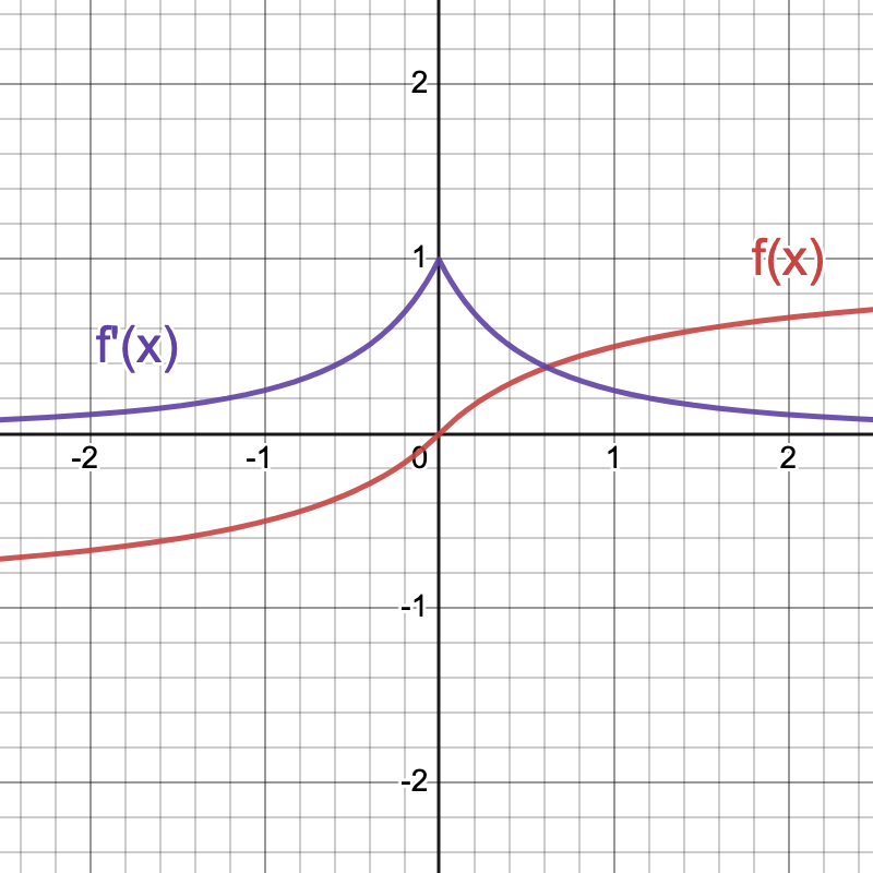
As can be observed, \(f^\prime(x)\) is not \(0\) everywhere and is maximum \(1\) at \(x=0\). Replacing the ill-defined \(\Theta^\prime(x)\) with \(f^\prime(x)\) and using it in conjunction with BPTT to directly train the SNNs is called the Surrogate Gradient Descent (SurrGD) method – as made popular by F. Zenke and E. Neftci.
Below is the code that enables the usage of surrogate-derivatives to directly train the SNNs via BPTT.
class SrgtDrtvSpike(torch.autograd.Function):
  """
  This class implements the spiking function for the forward pass along with its
  surrogate-derivative in the backward pass.
  """
  scale = 5

  @staticmethod
  def forward(ctx, x):
    """
    Computes the spikes and returns it.

    Args:
      ctx: is the context object.
      x: is the input of the spiking function - Heaviside step function. The input
        to this function should be `v(t) - v_thr`, i.e. S(v(t)) = H(v(t) - v_thr).
    """
    ctx.save_for_backward(x)
    out = torch.zeros_like(x)
    out[x >= 0] = 1.0
    return out

  @staticmethod
  def backward(ctx, grad_output):
    """
    Computes the local gradient to be propagated back. Note that the local
    gradient = gradient of the forward function * grad_output. Here the forward
    function is estimated as the fast sigmoid function: x/(1+|x|), whose gradient
    is 1/((1+|x|)^2).

    Args:
      ctx: is the context object whose stored values would be used to calculate
        local gradient.
      grad_output: is the gradient output received from the previous layer.
    """
    x, = ctx.saved_tensors
    grad_input = grad_output.clone()
    local_grad = grad_output * 1.0/((1.0 + torch.abs(x)*SrgtDrtvSpike.scale)**2)
    return local_grad

spike_func = SrgtDrtvSpike.apply
We use the spike_func defined above (via the class SrgtDrtvSpike) as the spiking function (in the spike_and_reset_voltage()) of the IF neurons, through which we want the error-gradients to flow backwards; thereby, enabling the training of network weights. We next define all the spiking layers to build our Dense-SNN.
Spiking Layers
Following are the implementations of the individual types of spiking layers in our Dense-SNN:
SpkEncoderLayer class
This class encodes the normalized pixel values to spikes via rate encoding, where the number of output spikes is proportional to the magnitude of the pixel value. An encoding neuron does this by implementing the following Current equation:
\[J = \nu \times x + \kappa\]where \(\nu\) and \(\kappa\) are the neuron’s gain and bias values respectively; \(x\) is the neuron’s input. Note that these \(\nu\) and \(\kappa\) values are neuron properties/hyper-parameters and can be tuned appropriately. Also note that I am not using the above-defined spike_func in the spike_and_reset_voltage() here, because the SpkEncoderLayer is the first layer in the network and there aren’t any trainable weights before this layer; thus, no need for the error-gradients to flow anymore backwards.
class SpkEncoderLayer(BaseSpkNeuron):
  def __init__(self, n_neurons, gain=1.0, bias=0.0):
    """
    Args:
      n_neurons: Number of spiking neurons.
      gain <int>: Gain value of the neuron.
      bias <int>: Bias value of the neuron.
    """
    super().__init__(n_neurons)
    self._gain = gain
    self._bias = bias

  def spike_and_reset_voltage(self):
    delta_v = self._v - self._v_thr
    spikes = torch.zeros_like(delta_v)
    spikes[delta_v >= 0] = 1.0
    self.reset_voltage(spikes)

    return spikes

  def encode(self, x_t):
    J = self._gain * x_t + self._bias
    self.update_voltage(J)
    spikes = self.spike_and_reset_voltage()

    return spikes
SpkHiddenLayer class
This class implements the hidden layer of IF neurons. Note that, to enable synaptic-weight learning in the hidden layers, I am using the spike_func defined above, which not only generates spikes in the forward pass but also facilitates error back-propagation via surrogate-derivatives in the backward pass.
class SpkHiddenLayer(BaseSpkNeuron, torch.nn.Module):
  def __init__(self, n_prev, n_hidn, dt=1e-3):
    """
    Args:
      n_prev <int>: Number of neurons in the previous layer.
      n_hidn <int>: Number of neurons in this hidden layer.
      dt <float>: Delta t to determine the current decay constant.
    """
    BaseSpkNeuron.__init__(self, n_hidn)
    torch.nn.Module.__init__(self)
    self._c = torch.zeros(BATCH_SIZE, n_hidn, device=DEVICE)
    self._c_decay = torch.as_tensor(np.exp(-dt/TAU_CUR))
    self._fc = torch.nn.Linear(n_prev, n_hidn, bias=False)
    self._fc.weight.data = torch.empty(
        n_hidn, n_prev, device=DEVICE).normal_(mean=0, std=2/np.sqrt(n_prev))

  def re_initialize_neuron_states(self):
    self.re_initialize_voltage()
    self._c = torch.zeros_like(self._c)

  def spike_and_reset_voltage(self): # Implement the abstract method.
    delta_v = self._v - self._v_thr
    spikes = spike_func(delta_v)
    self.reset_voltage(spikes)

    return spikes

  def forward(self, x_t):
    x_t = self._fc(x_t)
    self._c = self._c_decay*self._c + x_t
    self.update_voltage(self._c)
    spikes = self.spike_and_reset_voltage()

    return spikes
SpkOutputLayer class
This class is exactly the same as the SpkHiddenLayer class, except that the number of neurons is set equal to the number of classes in the dataset.
class SpkOutputLayer(SpkHiddenLayer):
  def __init__(self, n_prev, n_otp=10):
    """
    Args:
      n_prev <int>: Number of neurons in the previous layer.
      n_otp <int>: Number of classes in the output layer (or the dataset).
    """
    super().__init__(n_prev, n_otp)
Dense-SNN implementation
Now that we have all the constituent spiking layers ready, we can simply create our Dense-SNN. Architecturally, it has got one Encoder layer: SpkEncoderLayer class, two Hidden layers: one each of SpkHiddenLayer class, and one Output layer: SpkOutputLayer class.
class DenseSNN(torch.nn.Module):
  def __init__(self, n_ts):
    """
    Instantiates the DenseSNN class comprising of Spiking Encoder and Hidden
    layers.

    Args:
      n_ts <int>: Number of simualtion time-steps.
    """
    super().__init__()
    self.n_ts = n_ts
    self.enc_lyr = SpkEncoderLayer(n_neurons=784) # Image to Spike Encoder layer.
    self.hdn_lyrs = torch.nn.ModuleList()
    self.hdn_lyrs.append(SpkHiddenLayer(n_prev=784, n_hidn=1024)) # 1st Hidden Layer.
    self.hdn_lyrs.append(SpkHiddenLayer(n_prev=1024, n_hidn=512)) # 2nd Hidden Layer.
    self.otp_lyr = SpkOutputLayer(n_prev=512, n_otp=10)

  def _forward_through_time(self, x):
    """
    Implements the forward function through all the simulation time-steps.

    Args:
      x <Tensor>: Batch input of shape: (batch_size, 784). Note: 28x28 = 784.
    """
    all_ts_out_spks = torch.zeros(BATCH_SIZE, self.n_ts, 10) # #Classes = 10.
    for t in range(self.n_ts):
      spikes = self.enc_lyr.encode(x)
      for hdn_lyr in self.hdn_lyrs:
        spikes = hdn_lyr(spikes)
      spikes = self.otp_lyr(spikes)
      all_ts_out_spks[:, t] = spikes

    return all_ts_out_spks

  def forward(self, x):
    """
    Implements the forward function.

    Args:
      x <Tensor>: Batch input of shape: (batch_size, 784). Note: 28x28 = 784.
    """
    # Re-initialize the neuron states.
    self.enc_lyr.re_initialize_voltage()
    for hdn_lyr in self.hdn_lyrs:
      hdn_lyr.re_initialize_neuron_states()
    self.otp_lyr.re_initialize_neuron_states()

    # Do the forward pass through time, i.e., for all the simulation time-steps.
    all_ts_out_spks = self._forward_through_time(x)
    return all_ts_out_spks
For each input batch, the output spikes for all the simulation time-steps are collected in the all_ts_out_spks tensor. For computing training loss, the mean spike rate for all the output neurons will be obtained from all_ts_out_spks; the neuron with the highest firing rate is the predicted class. Note that for each input batch, the neuron sates of all the spiking layers are reintialized.
Training and Evaluation
We now directly train and evaluate our Dense-SNN on the MNIST dataset. Since the SNN here is a Dense-SNN with the input SpkEncoderLayer being a flat spiking layer, we have to flatten the MNIST images before feeding them to the SNN. Note that unlike the ANNs, the SNNs are inherently temporal and are supposed to be executed for a certain number of time-steps to build the neuron states and let them spike; this is done while training and inference as well. Therefore, I am setting the default number of simulation time-steps n_ts (or the presentation time) for each image as \(25\) time-steps. Increasing the presentation time can help increase the accuracy. To train the DenseSNN’s weights, I use the Adam optimizer via BPTT – i.e., internally, PyTorch unrolls the Dense-SNN in time and then back-propagates the error-gradients. The loss is defined on the mean firing rates of the SpkOutputLayer class neurons, using the CrossEntropyLoss function.
class TrainEvalDenseSNN(object):
  def __init__(self, n_ts=25, epochs=10):
    """
    Args:
      n_ts <int>: Number of time-steps to present each image for training/test.
      epochs <int>: Number of training epochs.
    """
    self.epochs = epochs
    self.loss_function = torch.nn.CrossEntropyLoss()
    self.model = DenseSNN(n_ts=n_ts).to(DEVICE) # n_ts = presentation time-steps.
    self.optimizer = torch.optim.Adam(self.model.parameters(), lr=1e-3)

    # Get the Train- and Test- Loader of the MNIST dataset.
    self.train_loader = torch.utils.data.DataLoader(
        torchvision.datasets.MNIST(root='./data', train=True, download=True,
                      transform=torchvision.transforms.Compose([
    # ToTensor transform automatically converts all image pixels in range [0, 1].
                          torchvision.transforms.ToTensor()
                          ])
                      ),
        batch_size=BATCH_SIZE, shuffle=True)
    self.test_loader = torch.utils.data.DataLoader(
        torchvision.datasets.MNIST(root='./data', train=False, download=True,
                       transform=torchvision.transforms.Compose([
    # ToTensor transform automatically converts all image pixels in range [0, 1].
                           torchvision.transforms.ToTensor()
                           ])
                      ),
        batch_size=BATCH_SIZE, shuffle=True)

  def train(self, epoch):
    all_true_ys, all_pred_ys = [], []
    all_batches_loss = []
    self.model.train()
    for trn_x, trn_y in self.train_loader:
      # Each batch trn_x and trn_y is of shape (BATCH_SIZE, 1, 28, 28) and
      # (BATCH_SIZE) respectively, where the image pixel values are between
      # [0, 1], and the image class is a numeral between [0, 9].
      trn_x = trn_x.flatten(start_dim=1).to(DEVICE) # Flatten from dim 1 onwards.
      all_ts_out_spks = self.model(trn_x) # Output = (BATCH_SIZE, n_ts, #Classes).
      mean_spk_rate_over_ts = torch.mean(all_ts_out_spks, axis=1) # Mean over time-steps.
      # Shape of mean_spk_rate_all_ts is (BATCH_SIZE, #Classes).
      trn_preds = torch.argmax(mean_spk_rate_over_ts, axis=1) # ArgMax over classes.
      # Shape of trn_preds is (BATCH_SIZE,).
      all_true_ys.extend(trn_y.detach().numpy().tolist())
      all_pred_ys.extend(trn_preds.detach().numpy().tolist())

      # Compute Training Loss and Back-propagate.
      loss_value = self.loss_function(mean_spk_rate_over_ts, trn_y)
      all_batches_loss.append(loss_value.detach().item())
      self.optimizer.zero_grad()
      loss_value.backward()
      self.optimizer.step()

    trn_accuracy = np.mean(np.array(all_true_ys) == np.array(all_pred_ys))
    return trn_accuracy, np.mean(all_batches_loss)

  def eval(self, epoch):
    all_true_ys, all_pred_ys = [], []
    self.model.eval()
    with torch.no_grad():
      for tst_x, tst_y in self.test_loader:
      # Each batch tst_x and tst_y is of shape (BATCH_SIZE, 1, 28, 28) and
      # (BATCH_SIZE) respectively, where the image pixel values are between
      # [0, 1], and the image class is a numeral between [0, 9].
        tst_x = tst_x.flatten(start_dim=1).to(DEVICE) # Flatten from dim 1 onwards.
        all_ts_out_spks = self.model(tst_x)
        mean_spk_rate_over_ts = torch.mean(all_ts_out_spks, axis=1)
        tst_preds = torch.argmax(mean_spk_rate_over_ts, axis=1)
        all_true_ys.append(tst_y.detach().numpy().tolist())
        all_pred_ys.append(tst_preds.detach().numpy().tolist())

    tst_accuracy = np.mean(np.array(all_true_ys) == np.array(all_pred_ys))
    return tst_accuracy

  def train_eval(self):
    for epoch in range(1, self.epochs+1):
      _, mean_loss = self.train(epoch)
      tst_accuracy = self.eval(epoch)
      print("Epoch: %s, Training Loss: %s, Test Accuracy: %s"
            % (epoch, mean_loss, tst_accuracy))
Now, we simply call the train_eval() of the above class TrainEvalDenseSNN to train and simultaneously evaluate our Dense-SNN on the entire test data every epoch.
trev_model = TrainEvalDenseSNN(n_ts=25, epochs=10)
trev_model.train_eval()
Epoch: 1, Training Loss: 1.6367219597101212, Test Accuracy: 0.9407
Epoch: 2, Training Loss: 1.53840385278066, Test Accuracy: 0.9554
Epoch: 3, Training Loss: 1.5242869714895884, Test Accuracy: 0.9621
Epoch: 4, Training Loss: 1.5161758770545324, Test Accuracy: 0.9664
Epoch: 5, Training Loss: 1.5111046055952708, Test Accuracy: 0.9703
Epoch: 6, Training Loss: 1.5074357161919276, Test Accuracy: 0.9715
Epoch: 7, Training Loss: 1.5046962410211564, Test Accuracy: 0.9736
Epoch: 8, Training Loss: 1.5025110612312953, Test Accuracy: 0.9751
Epoch: 9, Training Loss: 1.501358519991239, Test Accuracy: 0.9753
Epoch: 10, Training Loss: 1.4997689853111902, Test Accuracy: 0.975
Closing Words
As can be seen above, we obtained more than \(97\%\) test accuracy within \(10\) epochs on the MNIST dataset with just a simple Dense-SNN. A number of things can be done to improve the inference accuracy:
- Modify the network architecture – try incorporating
Convlayers - Increase the number of training epochs and/or the presentation time-steps
n_ts - Modify the
scalevariable in theSrgtDrtvSpikeclass - Try out other encoding mechanisms – different than rate encoding
- Try out different surrogate-derivative functions?
I highly encourage you to play with the scale variable in the SrgtDrtvSpike class, you would note that increasing it beyond a certain point is detrimental to the test accuracy. Why so? Think about it and report below in the comments!.
Hint - Plot the graph of the surrogate-derivative function \(\frac{1}{(1 + \gamma\times\text{abs}(x))^2}\), where \(\gamma\) is the
scaleand \(\text{abs}(.)\) is the absolute value (i.e., magnitude) function.
tags: tutorial - snns - surrogate-gradient-descent - surrogate-derivatives