Batchwise Training And Test Of Spiking Neural Networks For Image Classification In Nengo Dl

In this article, I will demonstrate how to train and test a 2D-CNN based image classification network using the Nengo-DL APIs, by passing the training/test data in batches.

By the end of this article, you will have learned

• How to use the scale_firing_rates parameter while training a Nengo-DL model?
• How to pass the training data in batches to train a model using the Nengo-DL APIs?
• How to pass the test data in batches while inferencing from a trained model using the Nengo-DL APIs?

A detailed previous article on building an SNN and inferencing from it already shows how to pass the test data in batches; if you haven’t gone through it, I highly recommend doing so. As shown in the linked article, to build an SNN, we first trained an ANN using the TensorFlow (TF) APIs and then converted it to an SNN using the nengo_dl.Converter() API. In this article though, we will use the Nengo-DL APIs (instead of the TF APIs) to train a Nengo-DL network. This is possible because Nengo-DL uses TF under the hood. By a Nengo-DL network, I still mean an ANN, and not an SNN. Directly training an SNN is still an active area of research (Wu et al., Pfeiffer et al., Lee et al., Lee at al., etc.). Bonus: An excellent tutorial on surrogate gradient descent for training SNNs can be be found here.

Sometimes, you may want to consider (or make use of) certain network-characteristics of a Nengo-DL network while training a model, e.g. the scale_firing_rates parameter; which isn’t natively possible with the TF APIs. Incorporating the scale_firing_rates parameter while training a network helps in the learning of weights which already account for the increase in neuron firing rates (when scaled later during inference). This may help in the SNNs having sparse activations (experimentally observed), resulting in lesser energy consumption when deployed on a neuromorphic hardware. Note that in the previous article, scale_firing_rates parameter was used only during the inference phase.

Also, it is possible that your training/test dataset is way too large to fit in its entirety in your GPU’s RAM. This would necessitate the need of a method to pass the training/test data in batches to the Nengo-DL model; this tutorial shows an example of it. Although the experiment here is done with the MNIST dataset, the method to pass data in batches can be extended to other large datasets as well.

This experiment’s environment was: tensorflow-gpu (v2.2.0), nengo (v3.1.0), and nengo_dl (v3.4.0); and my machine had a 12GB NVIDIA Tesla P100 GPU. You may have to adjust the values of train_batch_size and test_batch_size (in the code to follow) to suit the memory specifications of your machine’s GPU.

We will

• First build a 2D CNN based ANN using the TF APIs
• Then train it using the Nengo-DL APIs by passing the training data in batches
• Then evaluate the trained and converted model i.e. the SNN using the Nengo-DL APIs by passing the test data in batches

Let’s start coding!

# Importing Libraries
import matplotlib
import matplotlib.pyplot as plt
import nengo
import nengo_dl
import numpy as np
import sys
import tensorflow as tf

# Set memory growth of GPUs on your system.
gpus = tf.config.experimental.list_physical_devices("GPU")
for gpu in gpus:
  tf.config.experimental.set_memory_growth(gpu, True)

# Load the MNIST dataset.
(x_train, y_train), (x_test, y_test) = tf.keras.datasets.mnist.load_data()

# Binarize/One-Hot encode the training and test labels.
y_train = np.eye(10)[y_train].squeeze()
y_test = np.eye(10)[y_test].squeeze()

# Normalize the dataset.
x_train = x_train.astype(np.float32) / 127.5 - 1
x_test = x_test.astype(np.float32) / 127.5 - 1

Building the 2D CNN based ANN

We will reuse the network architecture introduced in the previous article, except that we will not regularize the kernels in the layers. This is because, if we include the kernel regularizers, it results into creation of “TensorNodes” in the SNN (obtained after conversion) which aren’t “Ensemble” objects in Nengo-DL. Ideally, we should not have any TensorNodes in our SNN, as the TensorNodes (in Nengo-DL) run on GPU and not on the neuromorphic hardware. Thus, not really offering any energy efficiency. On the other hand, the Ensembles run on neuromorphic hardware as they are composed of spiking neurons.

def get_2d_cnn_model(inpt_shape):
  """
  Returns a 2D-CNN model for image classification.

  Args:
    input_shape <tuple>: A tuple of 2D image shape e.g. (28, 28, 1)
  """
  def _get_cnn_block(layer, num_filters, layer_objs_lst):
    conv = tf.keras.layers.Conv2D(
        num_filters, 3, padding="same", activation="relu",
        kernel_initializer="he_uniform")(layer)
    avg_pool = tf.keras.layers.AveragePooling2D()(conv)

    layer_objs_lst.append(conv)
    return avg_pool

  layer_objs_lst = [] # To store the layer objects to probe later in Nengo-DL

  inpt_layer = tf.keras.Input(shape=inpt_shape)
  layer_objs_lst.append(inpt_layer)

  layer = _get_cnn_block(inpt_layer, 32, layer_objs_lst)
  layer = _get_cnn_block(layer, 64, layer_objs_lst)
  layer = _get_cnn_block(layer, 128, layer_objs_lst)

  flat = tf.keras.layers.Flatten()(layer)

  dense = tf.keras.layers.Dense(
      512, activation="relu", kernel_initializer="he_uniform")(flat)
  layer_objs_lst.append(dense)

  output_layer = tf.keras.layers.Dense(
      10, activation="softmax", kernel_initializer="he_uniform")(dense)
  layer_objs_lst.append(output_layer)

  model = tf.keras.Model(inputs=inpt_layer, outputs=output_layer)
  return model, layer_objs_lst

model, _ = get_2d_cnn_model((28, 28, 1))
model.summary()

Model: "model"
_________________________________________________________________
Layer (type)                 Output Shape              Param #
=================================================================
input_1 (InputLayer)         [(None, 28, 28, 1)]       0
_________________________________________________________________
conv2d (Conv2D)              (None, 28, 28, 32)        320
_________________________________________________________________
average_pooling2d (AveragePo (None, 14, 14, 32)        0
_________________________________________________________________
conv2d_1 (Conv2D)            (None, 14, 14, 64)        18496
_________________________________________________________________
average_pooling2d_1 (Average (None, 7, 7, 64)          0
_________________________________________________________________
conv2d_2 (Conv2D)            (None, 7, 7, 128)         73856
_________________________________________________________________
average_pooling2d_2 (Average (None, 3, 3, 128)         0
_________________________________________________________________
flatten (Flatten)            (None, 1152)              0
_________________________________________________________________
dense (Dense)                (None, 512)               590336
_________________________________________________________________
dense_1 (Dense)              (None, 10)                5130
=================================================================
Total params: 688,138
Trainable params: 688,138
Non-trainable params: 0
_________________________________________________________________

Let us print the network’s layers’ name, as well as their output shapes. This will be helpful while curating the training dataset in batches, where we need to mention the layers’ names as keys against matrices as values (defined later) in a dictionary.

print("2D-CNN model's layers' name...")
print("-"*50)
for index, layer in enumerate(model.layers):
  print(f"Layer ID {index} || and Layer name: {layer.name} || and output_shape: {layer.output_shape}")
print("-"*50)

2D-CNN model's layers' name...
--------------------------------------------------
Layer ID 0 || and Layer name: input_1 || and output_shape: [(None, 28, 28, 1)]
Layer ID 1 || and Layer name: conv2d || and output_shape: (None, 28, 28, 32)
Layer ID 2 || and Layer name: average_pooling2d || and output_shape: (None, 14, 14, 32)
Layer ID 3 || and Layer name: conv2d_1 || and output_shape: (None, 14, 14, 64)
Layer ID 4 || and Layer name: average_pooling2d_1 || and output_shape: (None, 7, 7, 64)
Layer ID 5 || and Layer name: conv2d_2 || and output_shape: (None, 7, 7, 128)
Layer ID 6 || and Layer name: average_pooling2d_2 || and output_shape: (None, 3, 3, 128)
Layer ID 7 || and Layer name: flatten || and output_shape: (None, 1152)
Layer ID 8 || and Layer name: dense || and output_shape: (None, 512)
Layer ID 9 || and Layer name: dense_1 || and output_shape: (None, 10)
--------------------------------------------------

Creating the Nengo-DL network

The following code creates and returns a Nengo-DL network; either an ANN or an SNN depending on value of mode (in the function below). Note that while training (i.e. mode = “train”), we do not replace the ReLU neurons with spiking neurons in the TF model while calling the nengo_dl.Converter() API, hence, an ANN is returned. However, while inferencing (i.e. mode = “test”), we replace the ReLU neurons with spiking neurons in the nengo_dl.Converter() API, hence, an SNN is returned.

Note that the scale_firing_rates parameter is assigned a value in both the modes.

def get_nengo_dl_model(sfr, mode):
  """
  Returns a Nengo-DL model for image classification.

  Args:
    sfr <int>: Value for the `scale_firing_rates` parameters.
    mode <str>: One of "train" or "test".
  """
  if mode != "train" and mode != "test":
    print(f"Wrong mode: {mode} while getting Nengo-DL model!! Exiting...")
    sys.exit()

  # MNIST has image shape: (28, 28, 1).
  model, layer_objs_lst = get_2d_cnn_model((28, 28, 1))

  if mode == "train":
    # Create the Nengo-DL network - a Nengo-DL wrapper over ANN here.
    # Note that we aren't replacing the ReLU neurons.
    np.random.seed(0)
    ndl_model = nengo_dl.Converter(
        model,
        scale_firing_rates=sfr
    )
  elif mode == "test":
    # Create the Nengo-DL network. Converting the ANN to SNN here.
    # Note that we are replacing the ReLU neurons with spiking ReLU.
    np.random.seed(0)
    ndl_model = nengo_dl.Converter(
        model,
        swap_activations={
            tf.keras.activations.relu: nengo.SpikingRectifiedLinear()},
        scale_firing_rates=sfr,
        synapse=0.005
    )

  # Get the probes for Input, first Conv, and the Output layers.
  ndl_probes = [ndl_model.inputs[layer_objs_lst[0]]] # Input layer probe.

  with ndl_model.net:
    nengo_dl.configure_settings(stateful=False) # Optimize simulation speed.
    # Probe for the first Conv layer.
    first_conv_probe = nengo.Probe(ndl_model.layers[layer_objs_lst[1]])
    ndl_probes.append(first_conv_probe)
    # Probe for penultimate dense layer.
    penltmt_dense_probe = nengo.Probe(ndl_model.layers[layer_objs_lst[-2]])
    ndl_probes.append(penltmt_dense_probe)

  ndl_probes.append(ndl_model.outputs[layer_objs_lst[-1]]) # Output layer probe.

  return ndl_model, ndl_probes

Curating the dataset

We use the MNIST dataset for our experiments. For such a small dataset, we really don’t need to create batches of training/test data. However, the code shown here to create batches and pass it to the Nengo-DL APIs can be extended to other large datasets as well.

For Training

While creating the batches of training data, we need to create two dictionaries: one for the input data (i.e. training images), and another for the output data (i.e. training labels). In the input dictionary, the keys are the layers’ name. The key with the model’s input layer’s name has training images’ data as value, and another key with the name “n_steps” has a matrix of ones as value (of shape: (batch_size, 1)) - we need to present the training images for only one time-step. These two keys are important and should be mentioned in the input dictionary. In case the model has layers with use_bias=True (which is “True” by default in the TF APIs for layers), we need to append those layers’ name with “.0.bias” and mention them as keys against matrices of ones as values (in fact, matrix values can be any, I chose ones). Those matrices are of shape (batch_size, number_of_channels, 1) for Conv layers, and of shape (batch_size, number_of_neurons, 1) for Dense layers. Note that such matrices are defined only for the layers with neurons.

For Inference

While creating the batches of test data for inference, it’s quite simple; we just create it as usual and then return it. We don’t need to create any dictionaries with custom values.

def get_batches_of_dataset(batch_size, n_steps, mode, layers=None):
  """
  Returns batches of NengoDL compatible training or test data.

  Args:
    batch_size <int>: Batch size of the training or test data.
    n_steps <int>: Number of time-steps an image is presented to the network.
    mode <str>: One of "train" or "test".
    layers <[]>: List of TensorFlow type layers.
  """
  if mode != "train" and mode != "test":
    print(f"Wrong mode: {mode} while curating dataset!! Exiting...")
    sys.exit()

  num_train_imgs, num_test_imgs = x_train.shape[0], x_test.shape[0]
  reshaped_x_train = x_train.reshape((num_train_imgs, 1, -1))
  reshaped_x_test = x_test.reshape((num_test_imgs, 1, -1))
  reshaped_y_train = y_train.reshape((num_train_imgs, 1, -1))

  if mode == "test":
    for start in range(0, num_test_imgs, batch_size):
      # Nengo-DL model complains if the batch_size of data is lesser than actual.
      if start+batch_size > num_test_imgs:
        continue

      # Tile the images, i.e. repeat each image `n_steps` number of times.
      tiled_x_test = np.tile(
          reshaped_x_test[start : start+batch_size], (1, n_steps, 1))
      yield (tiled_x_test, y_test[start : start+batch_size])

  elif mode == "train":
    # During training, since we train a non-spiking network,
    # we present the images only once.
    assert n_steps == 1
    for start in range(0, num_train_imgs, batch_size):
      tiled_x_train = np.tile( # n_steps = 1 here.
        reshaped_x_train[start : start+batch_size], (1, n_steps, 1))

      # Note that in the `input_dict` below there's no bias value mentioned for
      # the AveragePooling2D and Flatten Layers, as these layers have no neurons.
      input_dict = {
        layers[0].name: tiled_x_train, # Layer 0 is the input layer.
        # Next Conv layer has 32 channels.
        layers[1].name+".0.bias": np.ones((batch_size, 32, 1), dtype=np.int32),
        # Next Conv layer has 64 channels.
        layers[3].name+".0.bias": np.ones((batch_size, 64, 1), dtype=np.int32),
        # Next Conv layer has 128 channels.
        layers[5].name+".0.bias": np.ones((batch_size, 128, 1), dtype=np.int32),
        # Next Dense layer has 512 neurons.
        layers[8].name+".0.bias": np.ones((batch_size, 512, 1), dtype=np.int32),
        # Next Dense layer has 10 neurons.
        layers[9].name+".0.bias": np.ones((batch_size, 10, 1), dtype=np.int32),
        # Mention the value of n_steps parameter.
        "n_steps": np.ones((batch_size, 1), dtype=np.int32)
      }
      output_dict = {
        "probe": reshaped_y_train[start : start+batch_size]
      }

      yield (input_dict, output_dict)

Training the Nengo-DL Network

Next, we obtain the Nengo-DL network i.e. the ANN for training and train it via Nengo-DL APIs in a batchwise manner. For that, we can simply pass the training data generator (obtained from the get_batches_of_dataset() function above) to the fit() function of the Nengo-DL simulator object holding the network. We will then iteratively call the fit() function for a certain number of training epochs. Note the similarity of this Nengo-DL fit() function’s interface with that of the TF fit() function. After training the network, we will save the trained parameters, to be loaded later for inferencing.

sfr = 25
train_batch_size = 100
num_train_imgs = x_train.shape[0]
ndl_model, ndl_model_probes = get_nengo_dl_model(sfr, "train")

# Train the Nengo-DL Model.
with nengo_dl.Simulator(ndl_model.net, minibatch_size=train_batch_size, seed=0,
                        progress_bar=False) as ndl_sim:
  # Define the loss function applied at the output layer.
  losses = {
    ndl_model_probes[-1]: tf.losses.CategoricalCrossentropy()
  }
  # Compile the Nengo-DL model.
  ndl_sim.compile(
    optimizer=tf.optimizers.Adam(lr=0.001),
    loss=losses,
    metrics=["accuracy"]
  )
  ndl_model_layers = ndl_model.model.layers

  for epoch in range(8): # Train for 8 epochs.
    # Set n_steps=1 and mode="train" in the statment below for training.
    train_batches = get_batches_of_dataset(
        train_batch_size, 1, "train", ndl_model_layers)
    ndl_sim.fit(train_batches, epochs=1,
                steps_per_epoch=num_train_imgs//train_batch_size)

  # Save the trained network parameters.
  ndl_sim.save_params("nengo_dl_trained_model_params")

print("All Epochs Done! Training Completed.")

/home/rgaurav/miniconda3/envs/latest-nengo-tf/lib/python3.7/site-packages/nengo_dl/converter.py:588: UserWarning: Activation type <function softmax at 0x2b65ab157d40> does not have a native Nengo equivalent; falling back to a TensorNode
  "falling back to a TensorNode" % activation
/home/rgaurav/miniconda3/envs/latest-nengo-tf/lib/python3.7/site-packages/nengo_dl/simulator.py:1773: UserWarning: Number of elements (1) in ['str'] does not match number of Probes (3); consider using an explicit input dictionary in this case, so that the assignment of data to objects is unambiguous.
  len(objects),
2021-12-31 20:28:35.000233: W tensorflow/stream_executor/gpu/asm_compiler.cc:81] Running ptxas --version returned 256
2021-12-31 20:28:35.052992: W tensorflow/stream_executor/gpu/redzone_allocator.cc:314] Internal: ptxas exited with non-zero error code 256, output:
Relying on driver to perform ptx compilation.
Modify $PATH to customize ptxas location.
This message will be only logged once.


600/600 [==============================] - 6s 11ms/step - loss: 0.2237 - probe_loss: 0.2237 - probe_accuracy: 0.9338
600/600 [==============================] - 6s 10ms/step - loss: 0.0543 - probe_loss: 0.0543 - probe_accuracy: 0.9838
600/600 [==============================] - 6s 10ms/step - loss: 0.0366 - probe_loss: 0.0366 - probe_accuracy: 0.9893
600/600 [==============================] - 6s 10ms/step - loss: 0.0275 - probe_loss: 0.0275 - probe_accuracy: 0.9922
600/600 [==============================] - 6s 10ms/step - loss: 0.0224 - probe_loss: 0.0224 - probe_accuracy: 0.9933
600/600 [==============================] - 6s 10ms/step - loss: 0.0177 - probe_loss: 0.0177 - probe_accuracy: 0.9947
600/600 [==============================] - 6s 10ms/step - loss: 0.0139 - probe_loss: 0.0139 - probe_accuracy: 0.9956
600/600 [==============================] - 6s 10ms/step - loss: 0.0137 - probe_loss: 0.0137 - probe_accuracy: 0.9956
All Epochs Done! Training Completed.

After training for \(8\) epochs, I achieved a training accuracy of \(99.56\%\). You might get a similar accuracy score.

Inferencing from the Nengo-DL Network

Now that we have trained and saved the weights of the Nengo-DL network i.e. the ANN, let us convert it to an SNN. We can do this by simply replacing the ReLU neurons in the ANN with spiking ones; note that we also mention the synapse value as well as the scale_firing_rates value (in the nengo_dl.Converter() API in the get_nengo_dl_model() function) while converting to an SNN. We can then load the trained parameters into the SNN and predict on the test data passed in batches, and simultaneously collect the spikes and calculate accuracy. Note that to obtain a label for a test image, we need to execute the network for a certain number of time-steps for each image; this is taken care of while creating the test data - recollect tiling each test image. Here we execute the network for n_steps = \(60\) time-steps.

test_batch_size, test_acc, n_steps = 200, 0, 60
num_test_imgs = x_test.shape[0]
collect_spikes_output = True
ndl_mdl_spikes = [] # To store the spike outputs of the first Conv layer and the
                    # penultimate dense layer whose probes we defined earlier.
ndl_model, ndl_model_probes = get_nengo_dl_model(sfr, "test")
# Set n_steps=60 and mode="test" in the statment below for training.
test_batches = get_batches_of_dataset(test_batch_size, n_steps=n_steps, mode="test")

# Run the simulation for inference.
with nengo_dl.Simulator(ndl_model.net, minibatch_size=test_batch_size,
                        progress_bar=False) as ndl_sim:
  # Load the trained weights.
  ndl_sim.load_params("nengo_dl_trained_model_params")
  for batch in test_batches:
    # Pass the test data to the input layer, and predict on it.
    sim_data = ndl_sim.predict_on_batch({ndl_model_probes[0]: batch[0]})
    # Obtain predicted labels from last layer, and match it to the true labels.
    for y_true, y_pred in zip(batch[1], sim_data[ndl_model_probes[-1]]):
      if np.argmax(y_true) == np.argmax(y_pred[-1]):
        test_acc += 1

    # Collect the spikes if required.
    if collect_spikes_output:
      # Collecting spikes for each image in the first batch.
      for i in range(test_batch_size):
        ndl_mdl_spikes.append({
          ndl_model_probes[1].obj.ensemble.label: sim_data[ndl_model_probes[1]][i],
          ndl_model_probes[2].obj.ensemble.label: sim_data[ndl_model_probes[2]][i]
        })
      # Not collecting the spikes for rest of the batches to save memory.
      collect_spikes_output = False

print(f"Accuracy of the SNN over MNIST test images: {test_acc*100/num_test_imgs}")

Accuracy of the SNN over MNIST test images: 97.93

With our SNN, we achieve a test accuracy score of \(97.93\%\); you may obtain a similar score.

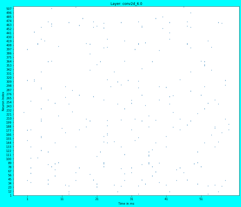
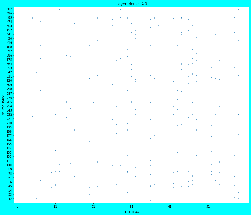
Plotting Spikes

We reuse the code from the previous article to plot the spikes obtained from the first Conv layer and the penultimate Dense layer of the SNN. In both the plots, note the sparsity of the spiking activity.

def plot_spikes(probe, test_data_idx=0, num_neurons=512, dt=0.001):
  """
  Plots the spikes of the layer corresponding to the `probe`.

  Args:
    probe <nengo.probe.Probe>: The probe object of the layer whose spikes are to
                               be plotted.
    test_data_idx <int>: Test image's index for which spikes were generated.
    num_neurons <int>: Number of random neurons for which spikes are to be plotted.
    dt <int>: The duration of each timestep. Nengo-DL's default duration is 0.001s.
  """
  lyr_name = probe.obj.ensemble.label
  spikes_matrix = ndl_mdl_spikes[test_data_idx][lyr_name] * sfr * dt
  neurons = np.random.choice(spikes_matrix.shape[1], num_neurons, replace=False)
  spikes_matrix = spikes_matrix[:, neurons]

  fig, ax = plt.subplots(figsize=(14, 12), facecolor="#00FFFF")
  color = matplotlib.cm.get_cmap('tab10')(0)
  timesteps = np.arange(n_steps)
  for i in range(num_neurons):
    for t in timesteps[np.where(spikes_matrix[:, i] != 0)]:
      ax.plot([t, t], [i+0.5, i+1.5], color=color)

  ax.set_ylim(0.5, num_neurons+0.5)
  ax.set_yticks(list(range(1, num_neurons+1, int(np.ceil(num_neurons/50)))))
  ax.set_xticks(list(range(1, n_steps+1, 10)))
  ax.set_ylabel("Neuron Index")
  ax.set_xlabel("Time in $ms$")
  ax.set_title("Layer: %s" % lyr_name)

Spike Plot of the first Conv layer

plot_spikes(ndl_model_probes[1]) # First Conv Layer.

Spike Plot of the penultimate Dense layer

plot_spikes(ndl_model_probes[2]) # Penultimate Dense Layer.

Analysis

In the previous article, we did not use the Nengo-DL APIs to train the ANN, rather used the TF APIs and then converted it to an SNN; while conversion for inference, we also scaled the neuron firing rates i.e. assigned a value to the scale_firing_rates parameter. We also saw that the first Conv layer’s spike plot was quite dense, although that was obtained with the CIFAR10 dataset. In case you run the previous article with the MNIST dataset, you will observe a similar dense spiking activity. Recollect that sparse spiking activity (and not dense) is desirable due to it consuming lesser energy.

In this article we observe that the spiking activity of the first Conv layer is quite sparse! Spiking activity plots of the deeper layers would be sparse as well, because they receive inputs from the previous layers. The sparsity in spiking activity is due to training the ANN using the Nengo-DL APIs in cognizance of the scale_firing_rates parameter (also, normalizing the dataset adds to the sparsity). In this case, Nengo-DL APIs consider the conversion of ANNs to SNNs beforehand and optimize the training process to create SNNs which better account for the dynamics of the spiking neurons, thus producing sparse activations. Although, we did not tune the scale_firing_rates parameter in this article, feel free to try out other values; in fact try out different values for training and inference. It is possible that if you do not set a value of the scale_firing_rates parameter while creating the Nengo-DL model for training, it would still produce a reasonably performing SNN (upon conversion) with sparse activations, however, a tuning might be necessary for a desired performance. Note that with the increase in the scale_firing_rates parameter value… although the test accuracy score would improve, spike activations may get denser. Also note that if the scale_firing_rates parameter isn’t mentioned in the nengo_dl.Converter() API, Nengo-DL assumes a value of \(1\) for it.

Well… this marks the end of this article, hope it was useful to you!

---