Spiking Neural Nets For Image Classification In Nengo Dl
by R Gaurav
In this blog article I will talk about building a Spiking Neural Network (SNN) for image classification using Nengo-DL - a python library for developing spiking neurons based deep learning models.
By the end of this article you will have learned:
- What are spiking networks? And why spiking networks?
- How to build spiking networks in Nengo-DL?
- How to do inference with spiking networks in Nengo-DL?
- How to visualize the neuron spikes?
Basic prior knowledge of spiking networks will be helpful, but not strictly required. Let’s begin by answering the first question.
What are spiking networks? And why spiking networks?
Spiking networks are the ones where the neuron activity computation is done via Spiking Neurons. For reference, my previous article gives a short introduction to the Spiking Neurons. In traditional Deep Learning models we have rate neurons e.g. ReLU, Sigmoid, etc. which output a real valued activation (e.g. \(0.56\)). That real valued activation is synonymous to the action-potential firing rate of biological neurons; and the artificial neurons which are implemented to fire action-potentials (or spikes) are called Spiking Neurons. Thus, neural network models built with spiking neurons are called Spiking Neural Networks (SNNs). Ohkay.. great! But why would we like to build SNNs when there are already best performing state-of-the-art rate neuron based models? That’s because, out of a number of advantages of spiking models, it offers us a software framework to leverage the low power Neuromorphic Hardware (which run spiking models) for deep learning tasks; thus helping us build low power AI models for energy critical applications, e.g. electric autonomous cars. And moreover, who wouldn’t like to save millions of joules of energy and contribute towards a green earth!
How to build spiking networks in Nengo-DL?
Before we proceed building our spiking network, let’s start with a short introduction to Nengo-DL. It is a relatively new Deep Learning (DL) library (actively developed and maintained by the Applied Brain Research team) for building spiking networks which can be deployed on low power Neuromorphic Hardware. For Deep Learning use cases, it currently (as of year \(2021\)) uses TensorFlow (TF) under the hood; and this provides it a great deal of power/flexibility in training and inferencing with rate neurons and spiking neurons respectively.
There are a number of ways to build spiking networks. Training with spiking neurons is difficult due to its non-differentiability and is also not scalable to deep networks (as of now). Therefore, we generally first train our network with rate neurons and then replace each rate neuron with its spiking equivalent (along with some other modifications in the network) to build a spiking model - to be run in inference mode. In short, with respect to Nengo-DL, we will here first build a TF network and then convert it to its spiking equivalent by using the API nengo_dl.Converter(model) where model is our TF rate neuron network.
The tutorial below was run on tensorflow-gpu (v\(2.2.0\)), nengo (v\(3.1.0\)), and nengo_dl (v\(3.4.0\)) and you will need these libraries to execute the code here. The installation instructions can be found here. Let’s begin with code now!
We will
- First build and train a TF network with ReLU neurons,
- Then convert it to a spiking network using
nengo_dl.Converter()API by replacing the ReLU neurons withnengo.SpikingRectifiedLinear()neurons and, - Then proceed with inference over the test data with the converted spiking network
We will use CIFAR-\(10\) dataset for our experiments. Note that I have experimented on \(12\)GB GPU machine, and you might need to alter the TF batch_size as well as the Nengo-DL batch_size depending upon your GPU resources.
Building a TF image classification 2D-CNN network
# Import libraries
import matplotlib
import matplotlib.pyplot as plt
import nengo
import nengo_dl
import numpy as np
import tensorflow as tf

# Set memory growth of GPUs on your system.
gpus = tf.config.experimental.list_physical_devices("GPU")
for gpu in gpus:
  tf.config.experimental.set_memory_growth(gpu, True)

# Load the CIFAR-10 dataset.
(x_train, y_train), (x_test, y_test) = tf.keras.datasets.cifar10.load_data()
class_names = ['airplane', 'automobile', 'bird', 'cat', 'deer',
               'dog', 'frog', 'horse', 'ship', 'truck']

# Binarize/One-Hot encode the training and test labels.
y_train = np.eye(10)[y_train].squeeze(axis=1)
y_test = np.eye(10)[y_test].squeeze(axis=1)
Now that we have loaded the data, we can proceed with building the TF 2D-CNN network.
def get_2d_cnn_model(inpt_shape):
  """
  Returns a 2D-CNN model for image classification.

  Args:
    input_shape <tuple>: A tuple of 2D image shape e.g. (32, 32, 3)
  """
  def _get_cnn_block(layer, num_filters, layer_objs_lst):
    conv = tf.keras.layers.Conv2D(
        num_filters, 3, padding="same", activation="relu",
        kernel_initializer="he_uniform",
        kernel_regularizer=tf.keras.regularizers.l2(0.005))(layer)
    avg_pool = tf.keras.layers.AveragePooling2D()(conv)

    layer_objs_lst.append(conv)
    return avg_pool

  layer_objs_lst = [] # To store the layer objects to probe later in Nengo-DL

  inpt_layer = tf.keras.Input(shape=inpt_shape)
  layer_objs_lst.append(inpt_layer)

  layer = _get_cnn_block(inpt_layer, 32, layer_objs_lst)
  layer = _get_cnn_block(layer, 64, layer_objs_lst)
  layer = _get_cnn_block(layer, 128, layer_objs_lst)

  flat = tf.keras.layers.Flatten()(layer)

  dense = tf.keras.layers.Dense(
      512, activation="relu", kernel_initializer="he_uniform",
      kernel_regularizer=tf.keras.regularizers.l2(0.005))(flat)
  layer_objs_lst.append(dense)

  output_layer = tf.keras.layers.Dense(
      10, activation="softmax", kernel_initializer="he_uniform",
      kernel_regularizer=tf.keras.regularizers.l2(0.005))(dense)
  layer_objs_lst.append(output_layer)

  model = tf.keras.Model(inputs=inpt_layer, outputs=output_layer)
  return model, layer_objs_lst
model, layer_objs_lst = get_2d_cnn_model((32, 32, 3))
model.summary()
model.compile(
    optimizer=tf.keras.optimizers.Adam(lr=0.001),
    loss="categorical_crossentropy",
    metrics=["accuracy"])
Training the TF network
Now that we have built and compiled our TF network, let’s proceed with batch training. Code to create the train/test data generator is below.
# Create the data generator for training and testing the TF network.
def get_data_generator(batch_size=128, is_train=True):
  """
  Returns a data generator.

  Args:
    batch_size <int>: Batch size of the data.
    is_train <bool>: Return a generator of training data if True
                     else of test data.
  """
  if is_train:
    for i in range(0, x_train.shape[0], batch_size):
      yield (x_train[i:i+batch_size], y_train[i:i+batch_size])
  else:
    for i in range(0, x_test.shape[0], batch_size):
      yield (x_test[i:i+batch_size], y_test[i:i+batch_size])

# Train the TF network.
for epoch in range(20):
  batches = get_data_generator()
  model.fit(batches)
After training the network for \(20\) epochs, I obtained a training accuracy of \(77.20\%\). You might get something similar. Let’s evaluate our TF network.
batches = get_data_generator(is_train=False)
results = model.evaluate(batches)
My TF network achieved an accuracy of \(71.11\%\) on the test data. Great! Now that we have trained our rate neuron based TF network and obtained a benchmark accuracy on the test data, we should next convert it to a spiking network and then evaluate it; as well as compare it against its TF equivalent.
Converting a TF trained network to Spiking Network
Converting a TF trained network to spiking network in Nengo-DL is as simple as calling the nengo_dl.Converter() API, but with proper arguments to it. Recollect that our TF network has ReLU neurons in its Convolutional and Dense layers (except the last output Dense layer which has softmax activation). As mentioned earlier, we need to replace the rate neurons (i.e. ReLU neurons here) with its spiking equivalent (nengo.SpikingRectifiedLinear() here) to build a spiking network. However, there lies more details to it than just swapping the neurons. Spiking networks are inherently temporal in nature. That is, they are supposed to execute for a (short) period of time to output meaningful results unlike the TF networks which output a desired value instantaneously. Why temporal nature? Because the spiking networks employ spiking neurons, and the spiking neurons produce spike (equivalent of an action potential) at specific timesteps only after receiving a required input over some time to reach their threshold, similar to how our biological neurons fire. Note that the modeled spikes are discrete and short-lived events. At this point you may want to go through my previous article on the operation of spiking neurons for a detailed understanding.
If the spiking networks execute over a period of time, at what instant of time do we consider it to have predicted the results? Answer: at the end of the simulation time. Ohkay… are we expecting “all” the spiking neurons to output a spike at the last instant of simulation? What if few neurons don’t spike at the last instant? Do we consider them to have ouput no result? Whoa.. that’s a lot of questions. Spiking neurons are not guaranteed to spike at each timestep during simulation. Therefore, we apply synpatic filtering to smooth the discrete spikes as well as to obtain a desired output value at each timestep during simulation. Thus, at the end of simulation, we have some output (which could be \(0\)) from each of the neurons. To leverage synaptic filtering we mention a non-zero value of synapse parameter in the nengo_dl.Converter() API. This value corresponds to the time constant of the default low pass filter in Nengo-DL. Note that a high synapse time constant will lead a spiking neuron to lag in reaching the expected output (with respect to the trained network) and a low synapse time constant will leave its output noisier.
Now, since the output of a spiking neuron depends upon its spike firing rate, what if the neurons fire spikes lazily (which could be due to a number of reasons, including the magnitude of the input value to it)? The output of the spiking neuron won’t be updated frequently, leading to a performance loss. This can be prevented by increasing the firing rate of spiking neurons, which can be done by mentioning a high value of scale_firing_rates parameter in the nengo_dl.Converter() API. Internally, Nengo-DL scales the input to the neurons by scale_firing_rates and then divides the output of the neurons by scale_firing_rates to maintain the same overall output (irrespective of scaling). As you may have guessed, this operation is valid only for the linear activation neurons (e.g. ReLU). Note that high scale_firing_rates value will… although result in spiking network behave similar to the rate network, it will lose the spiking benefit of low power Neuromorphic Hardware (due to high spiking activity) and small scale_firing_rates value will result in poor performance.
Now let’s build our spiking network. We will swap the ReLU neurons with nengo.SpikingRectifiedLinear() neurons, along with mentioning a synaptic time constant of \(0.005\) and set the scale_firing_rates parameter to \(20\). Following code does it.
# Get the spiking network.
sfr = 20
ndl_model = nengo_dl.Converter(
    model,
    swap_activations={
        tf.keras.activations.relu: nengo.SpikingRectifiedLinear()},
    scale_firing_rates=sfr,
    synapse=0.005,
    inference_only=True)
More details about the usage of nengo_dl.Converter() API, effects of its parameters, and much more can be found in this excellent tutorial. Note that here I am converting the TF trained model on the go, although you can also save the weights of the model and load it later, thereby calling the nengo_dl.Converter() API on it. Now that we have a trained spiking network ready, let’s proceed with inference.
How to do inference in Nengo-DL?
For inferencing with a Nengo-DL spiking network, as mentioned earlier, we need to execute it for a certain period of time and then look at the output of the network at the last timestep of the simulation (Note: For a robust output, you can as well take an average of the network’s output over a small window of the last few timesteps to smooth over the jittering effect). However, here too lies a small caveat; smaller simulation time will lead to poor performance and a large simulation time will deem the application of SNN ineffective due to latency in its predictions (although this would improve accuracy). For our purpose here, we will simulate the network for \(30\) timesteps (where each timestep is \(1ms\) by default in Nengo-DL), thus our image recognition model observes the input images for \(30ms\) of time before finally deciding on its label (note the similarity with the biological visual perception). To bring this into effect, we will have to tile each test image \(30\) times (done in the function get_nengo_compatible_test_data_generator() below).
# Tile the test images.
def get_nengo_compatible_test_data_generator(batch_size=100, n_steps=30):
  """
  Returns a test data generator of tiled (i.e. repeated) images.

  Args:
    batch_size <int>: Number of data elements in each batch.
    n_steps <int>: Number of timesteps for which the test data has to
                   be repeated.
  """
  num_images = x_test.shape[0]
  # Flatten the images
  reshaped_x_test = x_test.reshape((num_images, 1, -1))
  # Tile/Repeat them for `n_steps` times.
  tiled_x_test = np.tile(reshaped_x_test, (1, n_steps, 1))

  for i in range(0, num_images, batch_size):
    yield (tiled_x_test[i:i+batch_size], y_test[i:i+batch_size])
Now we have our trained spiking network in place along with the test data generator ready, let’s proceed with inference. However, let’s set up some probes first to feed in the batch-wise test images, receive the output predictions, and collect the spikes of the first convolutional layer and the penultimate dense layer. You can modify the code below to collect spikes of other layers too, but keep in mind that this will increase the memory consumption.
# Get the probes for Input, first Conv, and the Output layers.
ndl_mdl_inpt = ndl_model.inputs[layer_objs_lst[0]] # Input layer is Layer 0.
ndl_mdl_otpt = ndl_model.outputs[layer_objs_lst[-1]] # Output layer is last.
with ndl_model.net:
  nengo_dl.configure_settings(stateful=False) # Optimize simulation speed.
  # Probe for the first Conv layer.
  first_conv_probe = nengo.Probe(ndl_model.layers[layer_objs_lst[1]])
  # Probe for penultimate dense layer.
  penltmt_dense_probe = nengo.Probe(ndl_model.layers[layer_objs_lst[-2]])
Code to do inference in Nengo-DL
n_steps = 30 # Number of timesteps
batch_size = 100
collect_spikes_output = True
ndl_mdl_spikes = [] # To store the spike outputs of the first Conv layer and the
                    # penultimate dense layer whose probes we defined earlier.
ndl_mdl_otpt_cls_probs = [] # To store the true class labels and the temporal
                            # class-probabilities output of the model.

test_batches = get_nengo_compatible_test_data_generator(
    batch_size=batch_size, n_steps = n_steps)

# Run the simulation.
with nengo_dl.Simulator(ndl_model.net, minibatch_size=batch_size) as sim:
  # Predict on each batch.
  for batch in test_batches:
    sim_data = sim.predict_on_batch({ndl_mdl_inpt: batch[0]})
    for y_true, y_pred in zip(batch[1], sim_data[ndl_mdl_otpt]):
      # Note that y_true is an array of shape (10,) and y_pred is a matrix of
      # shape (n_steps, 10) where 10 is the number of classes in CIFAR-10 dataset.
      ndl_mdl_otpt_cls_probs.append((y_true, y_pred))

    # Collect the spikes if required.
    if collect_spikes_output:
      for i in range(batch_size): # Collecting spikes for each image in first batch.
        ndl_mdl_spikes.append({
          first_conv_probe.obj.ensemble.label: sim_data[first_conv_probe][i],
          penltmt_dense_probe.obj.ensemble.label: sim_data[penltmt_dense_probe][i]
        })
      # Not collecting the spikes for rest batches to save memory.
      collect_spikes_output = False
We are done with inference (using our spiking network) over the test data; let’s calculate our spiking network’s test accuracy. As mentioned above, the predicted classes y_pred for each test image is a matrix of temporally arranged class-probabilities, i.e. the spiking network outputs the class-probabilities of a test image at each timestep. In other words, the spiking model "thinks" what the test image could be… when it was allowed to see the image for a certain amount of time. After the end of the first timestep the predicted class-probabilities are obviously too immature to determine the correct label. Therefore, we generally consider the last timestep’s output to decide the predicted image label.
acc = 0
temporal_cls_probs = [] # To store the temporal class-probabilities of each test image.
for y_true, y_pred in ndl_mdl_otpt_cls_probs:
  # Pick the spiking network's last time-step output, therefore -1 in y_pred.
  temporal_cls_probs.append(y_pred)
  if np.argmax(y_true) == np.argmax(y_pred[-1]):
    acc += 1

print("Spiking network prediction accuracy: %s %%" % (acc * 100/ x_test.shape[0]))
Spiking network prediction accuracy: 61.71 %
We see that our spiking network’s test accuracy is close but not very close to the non-spiking TF model’s test accuracy. This is expected due to multiple reasons. Our spiking network is noisy and computation is discrete due to spikes. To reduce the effect of noise, one of the ways is to increase the synaptic time constant (try increasing the value of synapse to \(0.010\)). But keep in mind that consequently you would be required to simulate the network for a longer n_steps duration. You can also try increasing the scale_firing_rates parameter to \(50\) or so, or even simulate the above network as is for longer n_steps. With a particular combination of n_steps, synapse, and scale_firing_rates values we can achieve the non-spiking test accuracy, but is it worth it? The choice of these parameters depends upon your use case, thus it is a design problem. Increase in n_steps directly leads to increase in prediction latency, increase in scale_firing_rates directly leads to increase in power consumption (thus violating the purpose of using neuromorphic chips). Another way to achieve better test accuracy is to train ReLU neurons with noise added, but one has to be careful so as not to degrade the network semantics.
How to visualize the spikes?
We talked a lot about spikes. Now it’s time to visualize them. Note that according to the implementation of nengo.SpikingRectifiedLinear() neuron, it can output more than \(1\) spike in a single timestep. We however, are interested to just seeing the spikes; therefore, we will not consider the actual spike amplitudes, rather just the timesteps when they occur. Let’s plot the spikes collected from the first convolutional layer and the penultimate dense layer obtained from the simulation above. Note that I am not plotting the spiking neurons’ actual output values, you can do that by filtering the spikes.
def plot_spikes(probe, test_data_idx=0, num_neurons=512, dt=0.001):
  """
  Plots the spikes of the layer corresponding to the `probe`.

  Args:
    probe <nengo.probe.Probe>: The probe object of the layer whose spikes are to
                               be plotted.
    test_data_idx <int>: Test image's index for which spikes were generated.
    num_neurons <int>: Number of random neurons for which spikes are to be plotted.
    dt <int>: The duration of each timestep. Nengo-DL's default duration is 0.001s.
  """
  lyr_name = probe.obj.ensemble.label
  spikes_matrix = ndl_mdl_spikes[test_data_idx][lyr_name] * sfr * dt
  neurons = np.random.choice(spikes_matrix.shape[1], num_neurons, replace=False)
  spikes_matrix = spikes_matrix[:, neurons]

  fig, ax = plt.subplots(figsize=(14, 12), facecolor="#00FFFF")
  color = matplotlib.cm.get_cmap('tab10')(0)
  timesteps = np.arange(n_steps)
  for i in range(num_neurons):
    for t in timesteps[np.where(spikes_matrix[:, i] != 0)]:
      ax.plot([t, t], [i+0.5, i+1.5], color=color)

  ax.set_ylim(0.5, num_neurons+0.5)
  ax.set_yticks(list(range(1, num_neurons+1, int(np.ceil(num_neurons/50)))))
  ax.set_xticks(list(range(1, n_steps+1, 10)))
  ax.set_ylabel("Neuron Index")
  ax.set_xlabel("Time in $ms$")
  ax.set_title("Layer: %s" % lyr_name)
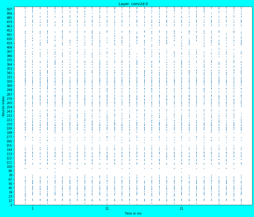
Spike plot for the first Convolutional layer is below.
plot_spikes(first_conv_probe)
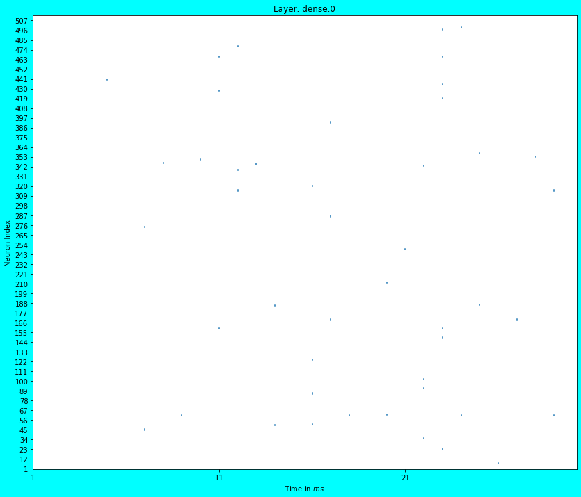
Spike plot for the penultimate dense layer is below.
plot_spikes(penltmt_dense_probe)
As can be seen in the above two plots for Layer conv2d.0 and dense.0, we see dots (which are actually small lines) which represent the spiking activity of \(512\) random neurons in the corresponding layers. The spiking activity is quite dense in the first Convolutional layer i.e. in conv2d.0. We see that most neurons in this layer spike every timestep. Is this good? or bad? It depends upon the design constraints. Ideally the spiking activity should be sparse for low power consumption.
Although in the penultimate dense layer’s spike plot i.e. in dense.0, we see the spiking activity is quite sparse. Good enough…, this layer consumes lesser power than layer conv2d.0. In spiking networks, you will generally find sparser spiking activity as you progress down the depth of the network. Most neurons don’t spike at deeper levels because they don’t get enough input from the previous layers; thus the spikes gradually die down as you go deeper (Note: If you add BatchNormalization layers, then you will note that the spiking activity is less sparse in deeper layers, however during conversion, the last mean/scaling terms used by BatchNormalization layers will be hard coded).
Visualizing the output layer class probabilities
As a means to close this article, let’s also plot how the class-probabilities vary with each timestep. I am plotting it for the test image at the indices \(0\) and \(19\) randomly. You can plot it for other test images too and observe the prediction behaviour with respect to timesteps.
def plot_probability(ax, true_cls, pred_cls, clss_probs, num_clss=10):
  """
  Plots the temporal variability in predicted class-probabilities.

  Args:
    ax <matplotlib.axes._subplots.AxesSubplot>: Subplot pane.
    true_cls <int>: The true class of the test image.
    pred_cls <int>: The predicted class of the test image from spiking network.
    clss_probs <numpy.ndarray>: The predicted class probabilities at each
                                timestep. Shape: (n_steps, num_clss).
  """
  ax.set_title("True Class: %s, Pred Class: %s" % (true_cls, pred_cls))
  ax.plot(clss_probs)
  ax.legend([str(j) for j in range(num_clss)], loc="upper left")
  ax.set_xlabel("Time in $ms$")
  ax.set_ylabel("Probability")
fig, axs = plt.subplots(1, 2, figsize=(16, 8), facecolor="#00FFFF")

# Plot for the test image at index 0.
plot_probability(
    axs[0],
    np.argmax(y_test[0]),
    np.argmax(temporal_cls_probs[0][-1]), # Last timestep's probability scores.
    temporal_cls_probs[0]
)

# Plot for the test image at index 19.
plot_probability(
    axs[1],
    np.argmax(y_test[19]),
    np.argmax(temporal_cls_probs[19][-1]), # Last timestep's probability scores.
    temporal_cls_probs[19]
)
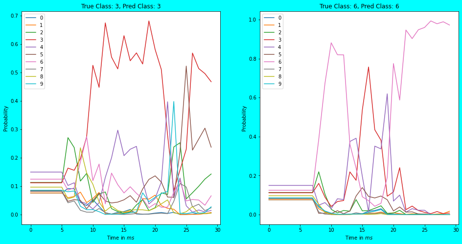
As can be seen in the above plots, the predicted class-probabilities vary at each timestep and tend to finalize at the last timestep. In the earlier timesteps (\(5ms\) to \(25ms\)) however, the predicted output is fuzzy and doesn’t even budge before \(5ms\) or \(7ms\) of time. With the chosen synapse = 0.005 and scale_firing_rates = 20, this naive spiking network recognizes \(61.71%\) percent of CIFAR-10 images correctly in n_steps = 30\(ms\) of time. Not bad!
Try playing with these above parameters to see their effects on the spike and class-probability plots. That’s it! Hope you found it useful :)
tags: blog - nengo-dl - snns - image-classification