Spiking Max Pooling In Convolutional Spiking Neural Networks
by R Gaurav
This article is about my research paper (accepted at IJCNN 2022) where two methods of spiking-MaxPooling in Convolutional Spiking Neural Networks (SNNs) are proposed; both these methods are entirely deployable on the Loihi neuromorphic hardware.
Learning objective:
- How to do spiking-MaxPooling in Convolutional SNNs?
This article only serves as a Proof-of-Concept (PoC) demonstration of the two proposed methods with minimal code to deploy them on Loihi. For more details on the entire suite of experiments, results, and analysis please go through the paper linked above. For the complete code of my experiments please visit my Github repo.
What’s the Problem Statement?
How to build Convolutional SNNs with MaxPooling layers such that they are entirely deployable on a neuromorphic hardware?
In the Convolutional SNNs (henceforth just SNNs here), MaxPooling isn’t as trivial as the regular \(max(.)\) operation. What will you take \(max(.)\) of? binary spikes? Will it be optimal? A few methods of MaxPooling in SNNs exist (more details in the paper linked above), but none of them have been evaluated on Loihi - in the context of MaxPooling in SNNs. Therefore, we designed two neurmorphic-hardware friendly methods of spiking-MaxPooling in SNNs, and evaluated their efficacy with a number of Image Classification experiments on MNIST, FMNIST, and CIFAR10 datasets.
Note that in the absence of such neuromorphic-hardware friendly spiking-MaxPooling methods, a lot of on-chip - off-chip inter-communication will happen upon the deployment of SNNs with MaxPooling layers on a neuromorphic hardware. This is due to the fact that the Conv layers with neurons get deployed on-chip and MaxPooling layers with no neurons get deployed off-chip. Such unsought inter-communication not only defeats the energy-efficiency motive of deploying SNNs on a neuromorphic hardware, but also results in spike-communication latency.
Methods of spiking-MaxPooling
I now present the theory and PoC demonstration of our proposed methods of spiking-MaxPooling, namely: MJOP and AVAM. Both of these methods rely on the representation of the artificial neuron activations as currents in the SNNs, obtained after filtering the spikes from the spiking neurons. Let’s consider the case of \(2\times2\) MaxPooling, where for one such pooling window, we need to find the \(max(U_1, U_2, U_3, U_4)\) where \(U_i\)s are the input current values. I used NengoLoihi backend to deploy both these methods - MJOP and AVAM on the Loihi neuromorphic hardware. For the benchmark purpose, I obtained the True Max U = \(max(U_1, U_2, U_3, U_4)\) from a different network run on CPU, and compared the outputs of the MJOP and AVAM methods with True Max U. The evaluation criterion is to visually check if the MJOP and AVAM outputs closely match the \(max(.)\) output!
MAX join-Op (MJOP)
The MJOP method of spiking-MaxPooling is a Loihi dependent method, as it uses the NxCore APIs and the Multi-Compartment (MC) neuron properties of Loihi. Note the subtle difference between “compartments” and “neurons”; a Loihi neuron can have one or more spiking units (called compartments) in it. MJOP method is loosely based on the simple observation that:
\[U_{max} = max(U_1, max(U_2, max(U_3, U_4)))\]Description
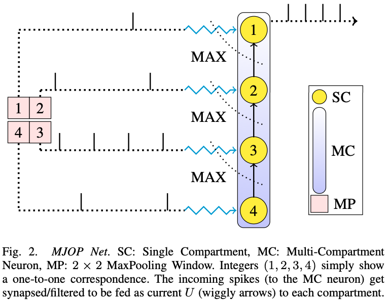
In a MC neuron, the Single-Compartment (SC) units are connected in a binary tree fashion, and can communicate the received \(U_i\) to their parent compartment. Note that each compartment in a MC neuron can be stimulated by an external input \(U_i\). Therefore, considering the case of a two compartment neuron i.e. the parent compartment has only one kid, where both the compartments receive currents \(U_1\) and \(U_2\) respectively, the parent compartment has to act on the current \(U_2\) from its kid. It does so by executing one of the many join operations provided by the low-level Loihi APIs. These join Ops can be MIN, ADD, MAX, etc.. And as you might have guessed by now, we used the MAX join-Op and the MC neuron creation functionality in Loihi to realize spiking-MaxPooling in SNNs - as shown in the figure below (for a \(2\times2\) MaxPooling window).
 |
|---|
| Fig taken from our paper - MJOP Net for \(2\times2\) MaxPooling |
The topmost root neuron receives a running \(max(.)\) of all the input currents, and then it spikes at a rate corresponding to the maximum computed current \(U_{max}\). Since it outputs spikes (and not the maximum current \(U_{max}\)) at a rate directly proportional to the maximum input current \(U_{max}\), we need to scale the filtered output spikes to match it to the true maximum current True Max U (note True Max U = \(U_{max}\)). Had the root neuron been able to communicate current to the next connected neuron on Loihi, outputting a simple \(max(.)\) of currents would have been possible; but this is not the case here. Note that, the required number of compartments in the MC neuron is same as the number of elements in the MaxPooling window. Also note that the value of scale depends on a number of factors, e.g. the root neuron’s configuration and the maximum input current to the root neuron. More details on how to choose the scale value are in our paper.
\(2\times2\) spiking-MaxPooling PoC Code
Since NengoLoihi uses the NxCore APIs (and not the NxNet APIs), I had to use the low level NxCore APIs to configure the Ensemble of neurons to a MC neuron on the Loihi hardware. In short, for a \(2\times2\) MaxPooling, you need to create an Ensemble of \(4\) neurons, then access the NengoLoihi object mapping the Ensemble to the Loihi board, and then configure the individual neurons (now considered as “compartments” on the Loihi board) to create a MC neuron with MAX join-Op between the compartments. I named such a network of compartments as the MJOP Net - in the figure above.
Following is the minimal PoC code for creating the MJOP Net:
def configure_ensemble_for_2x2_max_join_op(loihi_sim, ens):
  """
  Configures a Nengo Ensemble to create multiple Multi-Compartment Neurons with
  4 compartments and MAX join-Op between those compartments.

  Args:
    loihi_sim <nengo_loihi.simulator.Simulator>: NengoLoihi simulator object.
    ens <nengo.ensemble.Ensemble>: The Ensemble whose neurons are supposed to be
                                   configured.
  """

  nxsdk_board = loihi_sim.sims["loihi"].nxsdk_board
  board = loihi_sim.sims["loihi"].board

  # Get the blocks (which can be many depending on how large the Ensemble `ens`
  # is and in how many blocks is it broken).
  blocks = loihi_sim.model.objs[ens]
  #print("Number of (in and out) Blocks for Ensemble %s are: %s and %s."
  #          % (ens, len(blocks["in"]), len(blocks["out"])))
  for block in blocks["in"]:
    in_chip_idx, in_core_idx, in_block_idx, in_compartment_idxs, _ = (
        board.find_block(block))
    nxsdk_core = nxsdk_board.n2Chips[in_chip_idx].n2CoresAsList[in_core_idx]

    # Set the cxProfileCfg[0] as the leaf node's profile with `stackOut=3` =>
    # it pushes the current U to the top of the stack.
    nxsdk_core.cxProfileCfg[0].configure(stackOut=3, bapAction=0, refractDelay=0)
    # Set the cxProfileCfg[1] as the intermediate node's profile with `stackIn=2`
    # => it pops the element from the stack, `joinOp=2` => it does the MAX joinOp
    # with the popped element from stack and its current U, `stackOut=3` => it
    # pushes the MAXed current U on the top of the stack,
    # `decayU=nxsdk_core.cxProfileCfg[0].decayU` => the decay constant for current
    # U is same as that of the cxProfileCfg[0]. If `decayU` is 0, the current due
    # incoming spike never decays resulting in constant spiking of the neuron
    # and if it is default value, then the current decays instantly.
    nxsdk_core.cxProfileCfg[1].configure(
        stackIn=2, joinOp=2, stackOut=3, decayU=nxsdk_core.cxProfileCfg[0].decayU)
    # Set the root node which will output the spikes corresonding to the MAXed U.
    nxsdk_core.cxProfileCfg[2].configure(
        stackIn=2, joinOp=2, decayU=nxsdk_core.cxProfileCfg[0].decayU)

    # Set the compartments now.
    # Since the incoming connection from the previous Conv layer already as the
    # inputs in order of grouped slices, they are simply connected to the neuron
    # in this Ensembel `ens` from 0 index onwards.
    # `in_compartment_idxs` has the mapping of all compartment neurons in a
    # specific core, starting from index 0.

    # Maximum number of compartment idxs = 1024.
    for i in range(0, len(in_compartment_idxs), 4):
      c_idx = in_compartment_idxs[i]
      # Set a leaf node/compartment.
      nxsdk_core.cxCfg[c_idx].configure(cxProfile=0, vthProfile=0)
      # Set two intermediate nodes/compartments.
      nxsdk_core.cxCfg[c_idx+1].configure(cxProfile=1, vthProfile=0)
      nxsdk_core.cxCfg[c_idx+2].configure(cxProfile=1, vthProfile=0)
      # Set a root node/compartment to output spikes corresponding to MAX input.
      nxsdk_core.cxCfg[c_idx+3].configure(cxProfile=2, vthProfile=0)
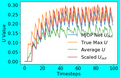
Following is the plot showing the scaled output from the MJOP Net compared to the True Max U.
 |
|---|
| MJOP Net PoC Plot |
Absolute Value based Associative Max (AVAM)
The AVAM method of spiking-MaxPooling is a neuromorphic-hardware independent method, such that it can be deployed on any hardware (CPU/GPU/Loihi etc.) which supports spiking neurons and the filtering of spikes. It is based on the following two equations:
\[max(a, b) = \frac{a+b}{2} + \frac{|a-b|}{2}\] \[max(a, b, c, d) = max(max(a, b), max(c, d))\]where \(a\), \(b\), \(c\), and \(d\) can be the currents \(U_1\), \(U_2\), \(U_3\), and \(U_4\) respectively, and |.| is the absolute value function. Note that the second equation can be extended to any number of arguments.
Description
The average term \(\frac{a+b}{2}\) can be easily implemented on Loihi, as it is a simple linear operation. Recollect that AveragePooling can be easily implemented through the weighted connections on Loihi. The challenge is to implement the non-linear absolute value function i.e. |.| on Loihi with the linear weighted connections and the non-linear spiking-neurons. How to do that?
| . | Approximation
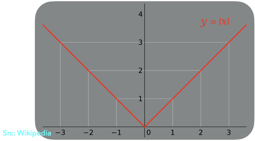
One fine day, while staring at the plot of |.| function (shown below), it struck to us that we can configure two spiking-neurons such that their Tuning Curves would look similar to the graph of |x|.
 |
|---|
| |x| Graph Plot |
What are the Tuning Curves?
Tuning Curves visually describe the activation profile of spiking neurons for an input stimulus.`
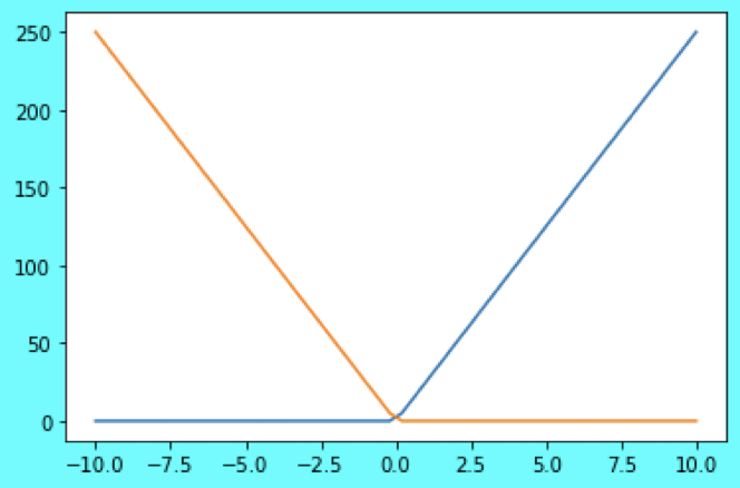
Therefore, we configured an Ensemble of two Integrate & Fire (IF) spiking neurons - one with a positive encoder value of \(1\), another with a negative encoder value of \(-1\) (figure below), i.e. one neuron fires for a positive input (while the other does not), and the another neuron fires for a negative input (while the other does not).
 |
|---|
| Tuning Curves Plot. x-axis -> Input, y-axis -> Output firing rate. For a negative input, the neuron with orange tuning curve spikes, neuron with blue tuning curve does not. Vice versa, for a positive input, neuron with blue tuning curve spikes, neuron with orange tuning curve does not. |
Note that, no matter the sign of the input, such a system of two neurons outputs a positive firing rate upon stimulated with a signed input. However, we need to normalize the output firing rate to obtain the absolute value of the input \(x\).
There’s a caveat though, for a near accurate approximation of |x|, the representational radius of the Ensemble neurons should be equal to the magnitude of the \(x\), i.e. radius = |x|. Whaaat?? How do we then set the radius parameter of the Ensemble of spiking neurons when we do not know what \(x\) will be? It turns out that for binary spiking neurons, there are some heuristics we can use to effectively set the radius value! More details about these heuristics can be found in our paper.
\(max(a, b)\) Approximation
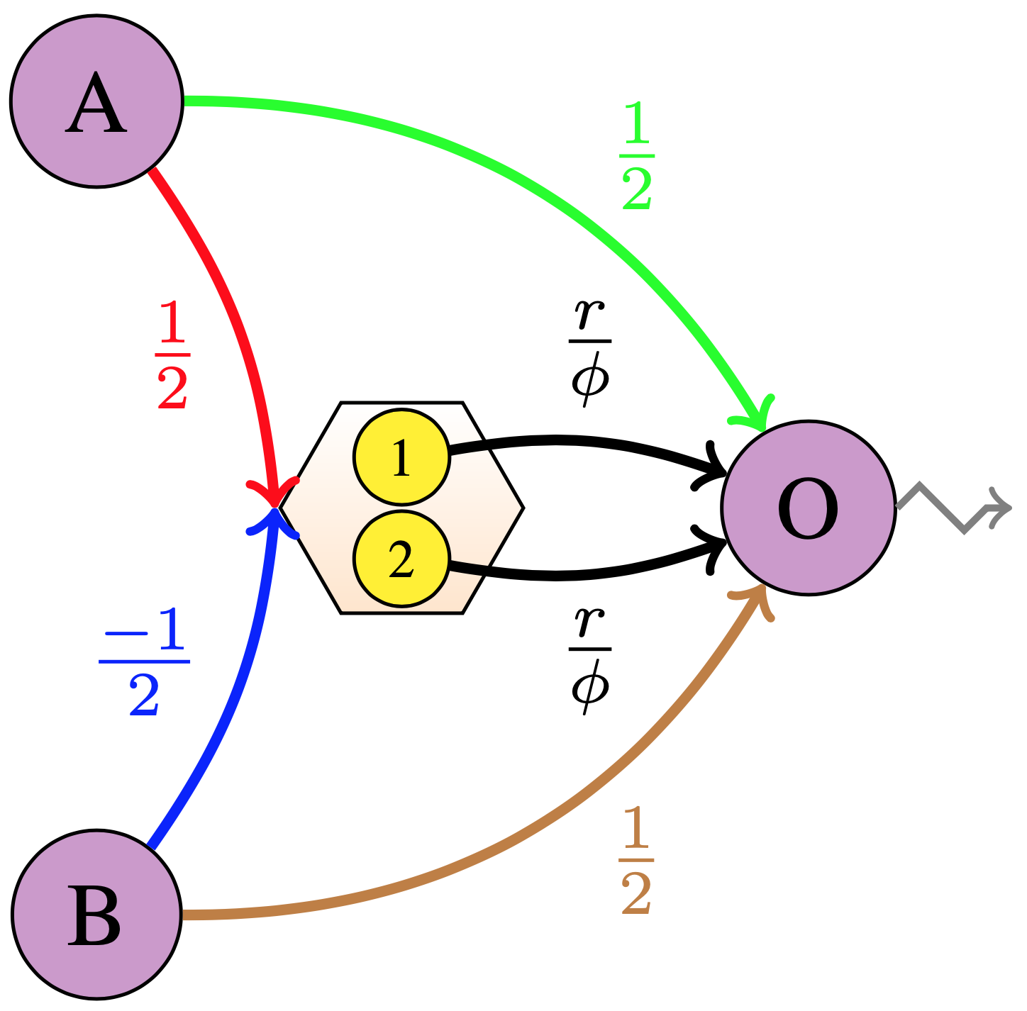
Combining the network representation for the linear average operation and the non-linear |.| operation, we obtain the following network - in the figure below, which quite well approximates the \(max(a, b)\) function.
 |
|---|
\(max(a, b)\) Network . \(r\) is the radius value, \(\phi\) is the maximum firing rate. Purple A and B are the input nodes, O is the output node. Yellow circles with numbers \(1\) and \(2\) are the IF spiking neurons. The output from the input nodes (A and B) are multiplied by \(\frac{1}{2}\) each and summed up at the output node (O) to get the average term \(\frac{a+b}{2}\). The output from the input nodes (A and B) also get multiplied by \(\frac{1}{2}\) and \(\frac{-1}{2}\) respectively to get the sum \(\frac{a-b}{2}\) input to the Ensemble of neurons. The output from the neurons is normalized with \(\phi\) and then multiplied by \(r\) to get the approximated \(\frac{|a-b|}{2}\), which is next added to the sum \(\frac{a+b}{2}\) at the output node (O) to finally output the approximated \(max(a, b)\). Note that only one of the two connections from the neurons to the output node (O) is active at a time, i.e. either the neuron \(1\) fires or the neuron \(2\) fires, not both. |
\(2\times2\) spiking-MaxPooling PoC Code
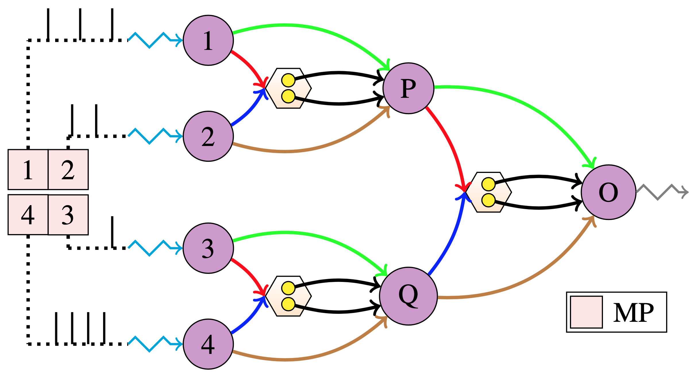
The above network for the \(max(a, b)\) can be hierarchically stacked to compute the \(max(a, b, c, d)\) as follows, in the figure below; I call such an hierarchical network as the AVAM Net.
 |
|---|
| Figure taken from our paper - AVAM Net created with stacked \(max(a, b)\) Network |
Following is the minimal PoC code for creating the AVAM Net:
def get_loihi_adapted_avam_net_for_2x2_max_pooling(
    seed=0, max_rate=500, radius=0.5, do_max=True, synapse=None):
  """
  Returns a Loihi adapted network for absolute value based associative max pooling.

  Args:
    seed <int>: Any arbitrary seed value.
    max_rate <int>: Max Firing rate of the neurons.
    radius <int>: Value at which Maximum Firing rate occurs (
                  i.e. the representational radius)
    do_max <bool>: Do MaxPooling if True else do AvgPooling.
    synapse <float>: Synapic time constant.
  """
  with nengo.Network(seed=seed) as net:
    net.inputs = nengo.Node(size_in=4) # 4 dimensional input for 2x2 MaxPooling.

    def _get_ensemble():
      ens =  nengo.Ensemble(
          n_neurons=2, dimensions=1, encoders=[[1], [-1]], intercepts=[0, 0],
          max_rates=[max_rate, max_rate], radius=radius,
          neuron_type=nengo_loihi.neurons.LoihiSpikingRectifiedLinear())
      return ens

    ens_12 = _get_ensemble() # Ensemble for max(a, b).
    ens_34 = _get_ensemble() # Ensemble for max(c, d).
    ens_1234 = _get_ensemble() # Ensemble for max(max(a, b), max(c, d)).

    # Intermediate passthrough nodes for summing and outputting the result.
    node_12 = nengo.Node(size_in=1) # For max(a, b).
    node_34 = nengo.Node(size_in=1) # For max(c, d).
    net.otp_node = nengo.Node(size_in=1) # For max(max(a, b), max(c, d)).

    ############################################################################
    # Calculate max(a, b) = (a+b)/2 + |a-b|/2.
    # Calculate (a+b)/2.
    nengo.Connection(net.inputs[0], node_12, synapse=None, transform=1/2)
    nengo.Connection(net.inputs[1], node_12, synapse=None, transform=1/2)

    if do_max:
      # Calculate |a-b|/2.
      nengo.Connection(net.inputs[0], ens_12, synapse=None, transform=1/2)
      nengo.Connection(net.inputs[1], ens_12, synapse=None, transform=-1/2)
      nengo.Connection(
          ens_12.neurons[0], node_12, synapse=synapse, transform=radius/max_rate)
      nengo.Connection(
          ens_12.neurons[1], node_12, synapse=synapse, transform=radius/max_rate)
    ############################################################################

    ############################################################################
    # Calculate max(c, d) = (c+d)/2 + |c-d|/2.
    # Calculate (c+d)/2.
    nengo.Connection(net.inputs[2], node_34, synapse=None, transform=1/2)
    nengo.Connection(net.inputs[3], node_34, synapse=None, transform=1/2)

    if do_max:
      # Calculate |c-d|/2.
      nengo.Connection(net.inputs[2], ens_34, synapse=None, transform=1/2)
      nengo.Connection(net.inputs[3], ens_34, synapse=None, transform=-1/2)
      nengo.Connection(
          ens_34.neurons[0], node_34, synapse=synapse, transform=radius/max_rate)
      nengo.Connection(
          ens_34.neurons[1], node_34, synapse=synapse, transform=radius/max_rate)
    ############################################################################

    ############################################################################
    # Calculate max(a, b, c, d) = max(max(a, b), max(c, d)).
    # Calculate (node_12 + node_34)/2.
    nengo.Connection(node_12, net.otp_node, synapse=synapse, transform=1/2)
    nengo.Connection(node_34, net.otp_node, synapse=synapse, transform=1/2)

    if do_max:
      # Calculate |node_12 - node_34|/2.
      nengo.Connection(node_12, ens_1234, synapse=synapse, transform=1/2)
      nengo.Connection(node_34, ens_1234, synapse=synapse, transform=-1/2)
      nengo.Connection(ens_1234.neurons[0], net.otp_node, synapse=synapse,
                       transform=radius/max_rate)
      nengo.Connection(ens_1234.neurons[1], net.otp_node, synapse=synapse,
                       transform=radius/max_rate)
    ############################################################################
  return net
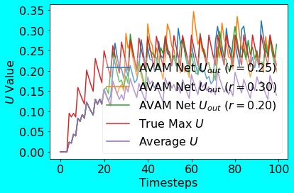
Following is the plot showing the outputs from the AVAM compared to the True Max U. Note that I have evaluated the AVAM Net for multiple radius values using the same input. Also note that for convenience purposes, I have kept the radius value same for the neurons in all the Ensembles.
 |
|---|
| AVAM Net PoC Plot |
Quick Analysis of the PoC plots
As can be seen from the above PoC output plots for both the methods, the MJOP Net’s scaled output closely matches the True Max U output. In case of the AVAM Net too, the outputs for different radius values closely matches the True Max U output; this implicitly shows the robustness of the AVAM Net w.r.t. the radius values. In the spirit of pooling methods, I also compared the AveragePooling output with that of the MJOP and AVAM Nets; as it can be seen, MJOP and AVAM outputs are higher than the AveragePooled output.
Closing Words
More details on how to adapt the MJOP and AVAM methods of spiking-MaxPooling in your SNNs can be found in our paper. I have evaluated MJOP and AVAM on Loihi-\(1\) only, so it will be interesting to see how these methods fare on Loihi-\(2\). I hope this PoC article helped you understand the crux of our paper. Please feel free to post your questions (if any) below!
tags: blog - nengo-loihi - snns - max-pooling - image-classification